Introduction
Monte Carlo Tree Search has been used for Connect 4, chess, Go, poker, and more. It can be applied to any game where a player selects from a finite number of available moves each turn.
Google used Monte Carlo Tree Search for its AlphaGo program. In 2016, this program beat the top Go player in the world.
This post explains:
- How and why Monte Carlo Tree Search works;
- How Google’s AlphaGo defeated the top Go player in the world; and
- The advantages and disadvantages of Monte Carlo Tree Search.
If you have not read the post on game trees and minimax, please consider reading it first. This post assumes that you are already familiar with game trees and minimax, and it probably won’t make much sense if you aren’t. It also assumes you are familiar with the terminology used to describe trees (e.g. root node, ancestor, descendant, leaf, etc.).
The MCTS Algorithm
Monte Carlo Tree Search (MCTS) has many similarities to the minimax technique described in the previous post: the Game Tree is similar and the logic for selecting moves is the same. But the estimated score for each node of the game tree does not come from an explicit score-estimation heuristic. Instead, the algorithm plays simulated games (called “playouts”) repeatedly, and it stores statistics about these playouts in the nodes of the game tree. MCTS uses these statistics to identify which move is best.
Overview
We will discuss each step in more detail below, but at a high level, the MCTS algorithm consists of the following three steps:
- Create a new leaf node of the game tree or select an existing leaf node of the game tree.
- Start with the game state represented by the leaf node from step 1. If this leaf node represents an in-progress game, simulate game moves until a win, loss, or draw is reached.
- Update the statistics of the leaf node and all of its ancestor nodes to reflect the outcome of the simulated game from step 2.
These three steps are repeated indefinitely. Step 1 almost always creates a new leaf node. Step 2 begins with the game state that the leaf node from step 1 represents, so almost every simulated game has a different starting point. The statistics derived from the simulations become more accurate as more simulations are performed.
Eventually, the programmer will stop the loop and look at the statistics it generated. The statistics will be used to select which move the computer will play.
We will discuss the three steps of the MCTS algorithm out of order. Step 1 (obtaining a leaf node) will be discussed last because it relies on the statistics that are generated in steps 2 and 3.
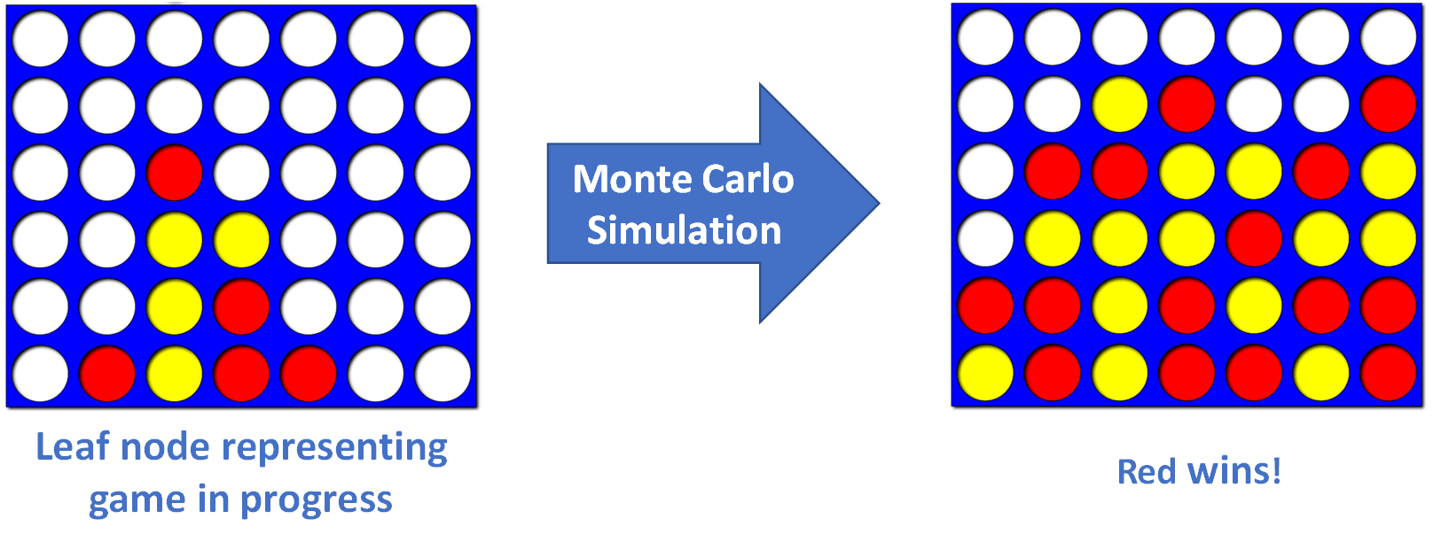
Step 2: Monte Carlo Simulation
MCTS always selects a leaf node of the game tree to simulate. (This is step 1, which we’ll discuss later.) The selected leaf node represents one of the many possible states of the game that may occur in the future. The purpose of the Monte Carlo simulation step is to estimate how often the game state represented by the selected leaf node results in a win.
Sometimes the selected leaf node represents a game that has completed. In this case, no simulation is necessary. We return an indication of whether the game resulted in a win, loss, or draw.
Most of the time the selected leaf node represents an in-progress game for which no win-rate statistics have been generated. To begin generating this information, we start with the game state the leaf node represents. We then simulate the remainder of the game and return the result of that simulation (i.e. win, loss, or draw). Only a single game is simulated.
Monte Carlo simulation
In the simplest case, the Monte Carlo simulation selects each remaining move in the game completely at random. For example, the simulation function used by the Connect 4 game on this site is:
function simulate(node: Node): GameStates {
    if (node.board.gameState == GameStates.Player1sTurn ||
        node.board.gameState == GameStates.Player2sTurn) {

        //make random moves to simulate remainder of game represented by node
        var board: Board = new boardClass(node.board);
        var moveIndex: number;
        while (board.gameState == GameStates.Player1sTurn ||
               board.gameState == GameStates.Player2sTurn) {
            moveIndex = Math.floor(Math.random() * board.availableMoves.length);
            board.makeMove(board.availableMoves[moveIndex]);
        }
        return board.gameState;

    } else {
        //nothing to simulate (node represents finished game)
        return node.board.gameState;
    }
}
This random simulation strategy is best when the programmer does not know how to model the opponent’s play, or where the best model of the opponent’s play really is random.
MCTS focuses its search of the game tree on the moves with the best simulation results. If the simulation results accurately represent an opponent’s play, MCTS can focus its search on the moves its opponent is most likely to make. For this reason, Google’s AlphaGo simulates the game play of human experts when performing simulations.1
Step 3: Updating Statistics
Each node of the game tree stores the number of simulations that have been run that include this node’s game state and a tally of the results of those simulations. These two numbers can be combined to indicate this node’s win rate—the percentage of the time this node’s game state results in a win.
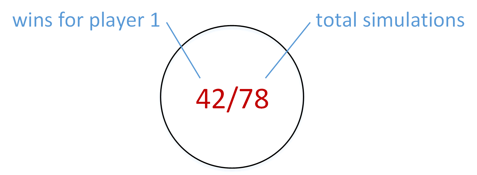
A node with a win rate for player 1 of 42/78=54%
Simulations are always run on a leaf node of the game tree. Each simulation result is stored in the relevant leaf. The simulation result is also stored in each ancestor of the leaf that was simulated. This is done because these ancestor nodes represent earlier stages of the game that was simulated. Figure 3 illustrates the process of updating the game tree to reflect a new simulation result.
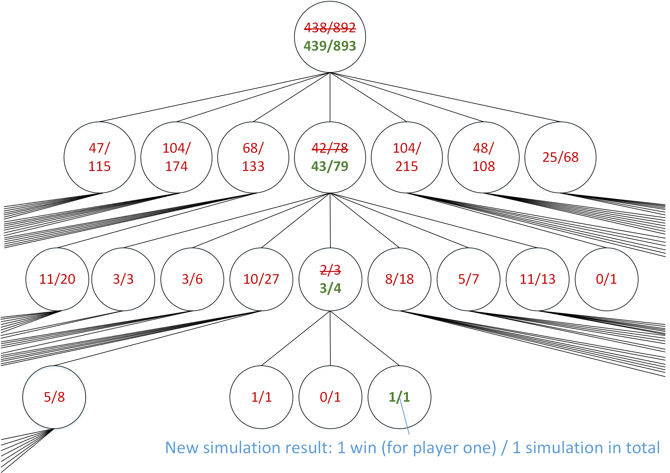
Green text indicates statistics updated to reflect one new simulation that resulted in a win.
Example code that updates the tree in this manner is provided below.
function updateStats(leaf: Node, simResult: GameStates): void {
    var curr: Node = leaf;
    while (curr) {
        if (simResult == GameStates.Player1Wins) {
            curr.p1winTally += 1;
        } else if (simResult == GameStates.Draw) {
            curr.p1winTally += 0.5;
        }
        curr.totalSimulations += 1;
        curr = curr.parent;
    }
}
Step 1: Obtaining a Leaf Node to Simulate
Now that we have discussed what happens to each leaf node that is identified for a Monte Carlo simulation, let’s return to step 1 and discuss how that leaf node was obtained.
The MCTS algorithm begins at the top of the tree (at the root node). It gives a score to each child node of this node, and it picks the child with the highest score. For purposes of this discussion, we’ll call giving each child of a node a score and picking the child with highest score pick best child. The details of how pick best child assigns scores will be discussed in the next section.
Pick best child is run repeatedly. Each time, it starts from the node that was last picked. It gives each child of that node a score, and it picks the one with the highest score. The process stops when a node with zero children or with missing children is picked.
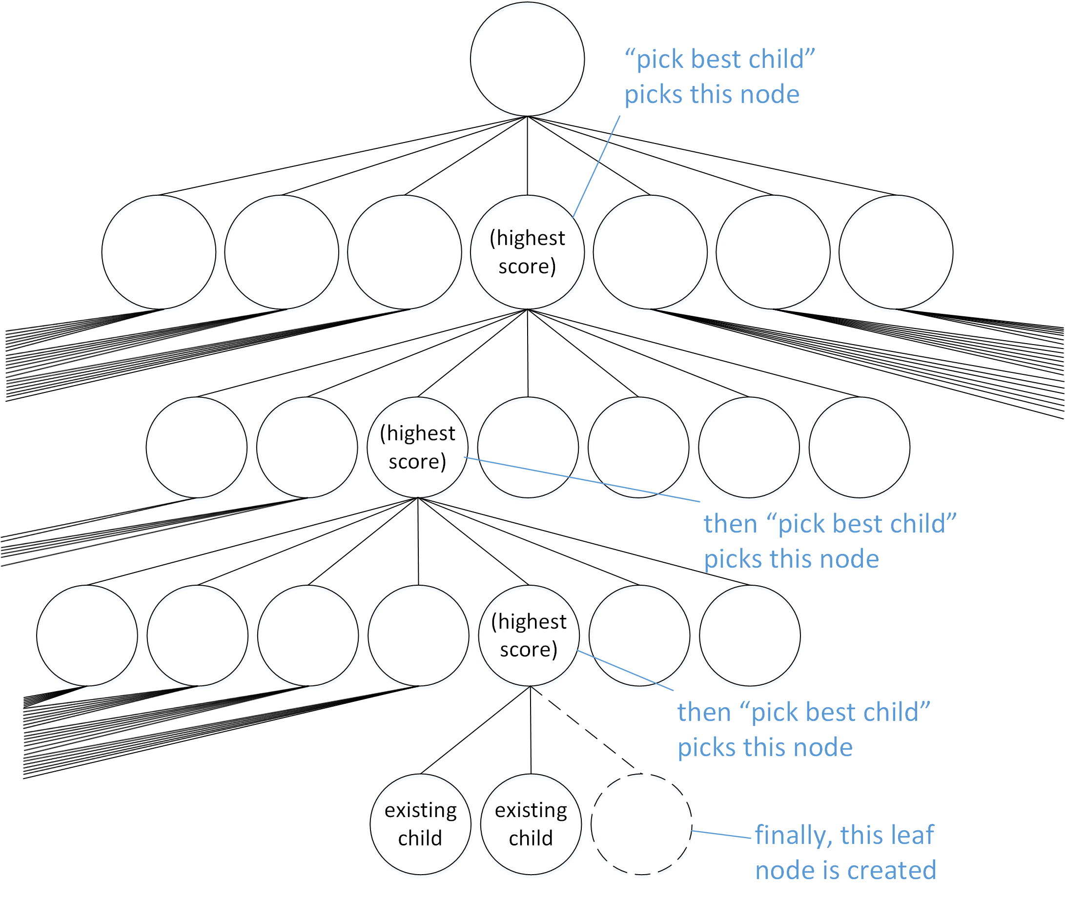
Pick best child descends down the game tree until a node with missing children is reached
If the node pick best child picks is missing children, one of the missing children will be created. The newly-created leaf node is the one that is used by steps 2 and 3 (discussed above) to run a simulation and update the statistics. If this process encounters a node that has zero children because it represents the end of a game (a win, loss, or draw), then it is not possible to create a child. Consequently, the node with zero children is the one used by steps 2 and 3.
An example of code that implements this process is:
function getNodeToSimulate(root: Node): Node {
    var curr: Node = root;

    while ( canHaveChildren(curr) ) {
        if ( missingChildren(curr) )  {
            return createMissingChild(curr);

        } else { //all children of curr exist, so descend down the tree
            curr = pickBestChild(curr);
        }
    }
    return curr;//curr is a win, loss, or draw (no children possible)
}
How Scores Are Assigned
As described above, pick best child descends down the game tree in search of the leaf node to use for the next simulation. We want it to focus on the most promising game moves—those that have the best win statistics. But we need to avoid relying too heavily on the win statistics because they may be inaccurate.
For example, assume we have simulated one move ten times, finding that it resulted in a win five of those times. Assume we simulated a second move ten times, finding that it resulted in a win four of those times. In this scenario, we should not attribute much significance to the first move’s win rate being 10% higher than the second move’s win rate. That 10% difference is within the margin of error, and we really don’t know which move is better yet. In short, it’s too early to focus on only one of these moves. Instead, we need to explore the descendants of both of these nodes.
Conversely, if we have simulated both moves many thousands of times, and there is still a 10% difference in the win rate, we now have some confidence that the move with the higher win rate is in fact better. In this situation we have explored enough, and it now makes sense to focus on exploiting our results. We do this by focusing our remaining exploration and expansion of the game tree on the descendants of the most promising node.
We represent these intuitions mathematically using the formula below. Recall that pick best child starts from a parent node, scores all its children, and selects the child with the highest score. Each score is calculated as follows:
$$Score = Win Rate + c \cdot \sqrt{ \frac{2 \cdot \ln{Parent Simulations}}{Node Simulations} }$$
$Win Rate$ is the percentage of simulations that were won by the player whose turn it is.
$Parent Simulations$ is the number of simulations that include the game state of the parent node.
$Node Simulations$ is the number of simulations that include the game state of the child node being scored.
The first portion of the score ($Win Rate$) has a value between 0 and 1. If it is the first player’s turn, the win rate reflects how often the first player won the simulations. If it is the second player’s turn, the win rate reflects how often the second player won the simulations. The win rate portion of the score encourages selection of the option that is most promising to the current player, since that is what a savvy player is most likely to select.
The second portion of the score ($c \cdot \sqrt{ \frac{2 \cdot \ln{Parent Simulations}}{Node Simulations} }$) represents how important it is to explore this node. This term has a relatively high value at first. But it decreases towards zero the more times the node has been simulated. $c$ is a constant that can be used to tune amount of emphasis put on exploration vs. exploitation. $c=1$ appears in the literature,2 but higher values are appropriate for situations where the algorithm may be run for only a short time or where early simulation results may be inaccurate.
Figure 5 illustrates the how this scoring system encourages exploration. In Figure 5, the node on the left has a win rate of 50%, and the node on the right has a win rate of only 30%. Thus, the node on the left seems much more promising. But the score for the node on the right is higher, meaning that it is more important to run a simulation on a descendant of the right node than the left node. This occurred because the node on the right has only been simulated 100 times, whereas the node on the left has been simulated 1,000 times. Once the node on the right has been simulated thousands of times, it will receive a much smaller boost from the $c \cdot \sqrt{ \frac{2 \cdot \ln{Parent Simulations}}{Node Simulations} }$ term, and the $Win Rate$ will become the largest component of its score.
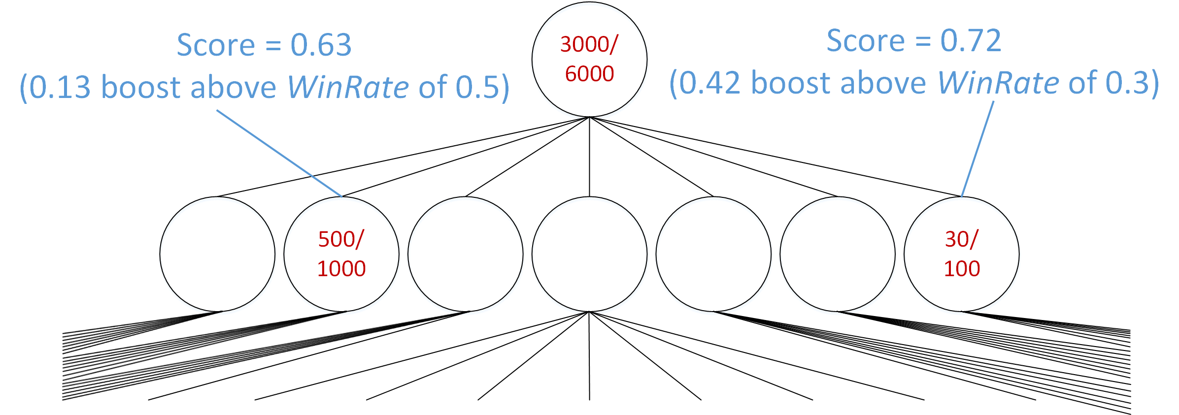
The $c \cdot \sqrt{ \frac{2 \cdot \ln{Parent Simulations}}{Node Simulations} }$ term boosts the score of a node with only 100 simulations above the score of a node with 1,000 simulations.
Selecting A Move
When choosing which move to play in the real game (as opposed to in simulation), there is no benefit to exploration. The move with the highest $Win Rate$ is selected.
Why It Works
No node is selected for Monte Carlo simulation twice unless it represents the end of a game (i.e. a win, loss, or draw). For each node that represents an in-progress game, the vast majority of its simulation statistics come from simulations run on its descendants. In these descendant nodes, many of the moves were selected by pick best child using the scoring system described above.
After the initial exploration has died down, the moves selected by the scoring system represent the best game play that has been discovered. Indeed, pick best child uses the same logic as the minimax move selection algorithm: that each player will make the move that maximizes his own win rate. Since pick best child focuses on the best-known sequence of upcoming moves, those optimal moves dominate the simulation statistics.
In essence, MCTS pulls itself up by its bootstraps. It starts with the relatively-poor results of initial simulated game play. But it continually improves on these results by expanding the most promising portions of the game tree and adding results from these more-optimal branches. Given enough time, the simulation results converge to values that will allow for perfect game play.3
Alpha Go
AlphaGo beat the reigning Go champion in 2016.4 It used two tweaks to the MCTS algorithm.5
Alpha Go’s Monte Carlo Simulations
Google’s AlphaGo does not simulate game play using random moves. Instead, it uses a neural network that was trained to simulate the moves of human experts.
AlphaGo also uses a separate neural network to predict the outcome of a game. This is similar to the score-estimating heuristics used with traditional minimax algorithms. AlphaGo averages the output of its outcome-prediction neural network with the outcome of the simulated game play.6 It returns this combined value as the result of each simulation.
AlphaGo’s Identification of Nodes to Simulate
When AlphaGo travels down the game tree in search of the next node to expand and simulate, it uses a slightly different equation to score each of the child nodes under consideration. Instead of:
$$Score = Win Rate + c \cdot \sqrt{ \frac{2 \cdot \ln{Parent Simulations}}{Node Simulations} }$$
AlphaGo uses:
$$Score = Win Rate + c \cdot \frac{Prior Probability}{1+Node Simulations} $$
$Prior Probability$ is a number that indicates the likelihood of this move being made by a human. It comes from a neural network that Google trained based on “expert human moves.”
Both of these equations are similar in that the second term encourages exploration at first, but it decreases to insignificance once the node has been simulated a large number of times.
The difference is that AlphaGo does not treat each child node equally when it encourages exploration. Instead, exploration is weighted towards the moves the neural network thinks are most likely.
Comparison to Traditional Techniques
No Heuristics Needed
Unlike traditional minimax techniques, MCTS does not need to rely on an explicit score-estimating heuristic. Instead, MCTS can discover for itself how to play a game well. In fact, the probability of MCTS selecting the optimal move converges to 100% the longer the algorithm runs.7
Not Best for Every Game
Although MCTS has proven to be useful for Go, it is slower than traditional minimax techniques for Chess. This is because Chess has many situations where the best initial move results in success only when it is followed by a very specific series of subsequent moves, but the average series of subsequent moves has poor results. In these situations, MCTS focuses its initial efforts on other moves. It doesn’t focus on the best initial move until after it discovers the specific series of subsequent moves that results in success.
Continual Improvement
MCTS can return a recommended move at any time because the statistics about the simulated games are constantly updated. The recommended moves aren’t great when the algorithm starts, but they continually improve as the algorithm runs.
Traditional minimax algorithms, on the other hand, can only update the recommend move after the game tree has been expanded by a preset amount, estimated scores have been assigned to the leaf nodes, and those estimated scores have been used to calculate new estimated scores for the remaining nodes.
This difference is particularly important for software that may be run in unknown environments. Users expect a quick result, regardless of the speed of their computer (or phone) and regardless of whether a virus scan or compiler is running in the background.
MCTS’s continual improvement over time can also be exploited to make the algorithm play a game at varying levels of competency. Lower difficulty levels are achieved by stopping the algorithm before it has a chance to improve the initial set of recommended moves.
Conclusion
Thanks for reading! I hope you now have a better understanding of MCTS—the algorithm that simulates game play in order to identify the best game move to make. Click here to see MCTS in action.
-
The strategy used by AlphaGo is discussed in more detail at the end of this post. ↩︎
-
L. Kocsis, C. Szepesvari, “Bandit based Monte-Carlo Planning,” in Euro. Conf. Mach. Learn. Berlin, Germany: Springer, 2006, pp. 282-293. Available here. Note that the paper uses a slightly different form of the equation. ↩︎
-
L. Kocsis, C. Szepesvari, J. Willemson, “Improved Monte-Carlo Search,” Univ. Tartu, Estonia, Tech. Rep. 1, 2006. (Available here.) ↩︎
-
My information about AlphaGo comes from D. Silver, et al., Mastering the game of Go with deep neural networks and tree search, Nature, 2016. ↩︎
-
There are several variants of AlphaGo. Some variants return only the neural network’s estimate of the game’s outcome. Other variants return only the result of simulated game play. Google reported the best results when returning the average of these two values. ↩︎
-
L. Kocsis, C. Szepesvari, J. Willemson, “Improved Monte-Carlo Search,” Univ. Tartu, Estonia, Tech. Rep. 1, 2006. (Available here.) ↩︎