Introduction
IBM’s Deep Blue beat the reigning world chess champion. This is old news. It occurred in 1997. But the techniques IBM used to achieve this result are still the best ones known for Chess. Indeed, these same techniques are still used by today’s leading computer chess engines.
This post will explain:
- How to make a computer play a game perfectly;
- Why perfect play is impossible to achieve in practice; and
- How IBM’s Deep Blue defeated the reigning chess champion.
The information in this post is fundamental to understanding the next post, which explains the algorithm used by programs such as Google’s AlphaGo to play the game Go.
Let’s get started.
Game Trees
Any game where a player selects from a finite number of available moves each turn can be represented using a game tree. Each node in the tree represents a state of the game, and each vertex represents a possible move that can be made. For example, Connect 4 starts with an empty board, so the root of the tree is an empty board. The first player can place his piece in one of seven possible positions, so the root has seven children, each representing one of the seven possible moves.
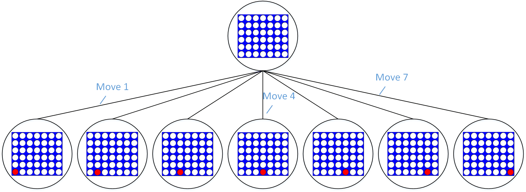
The beginning of a game tree
After the first player makes a move, the second player can place a game piece in one of seven possible positions. Thus, each of the child nodes from Figure 1 also has seven children, as illustrated in Figure 2.
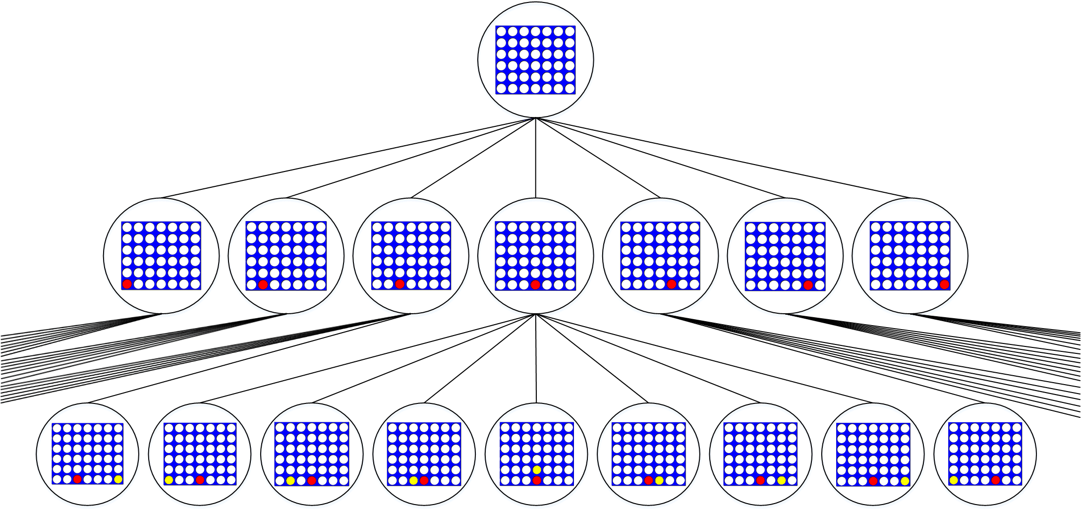
The second row of the game tree has 7*7=49 nodes (most of which do not fit on the screen).
Of course, the game is not over yet, so each of these nodes have seven children, each of those children have seven children of their own, and so on. The only nodes that do not have any children are nodes that represent the end of the game (e.g. a win, loss, or tie). As you can see, the game tree quickly becomes very large. Game-playing AI’s have several techniques for limiting the size of the game tree that needs to be stored in memory. But before we can understand them we need to consider how moves are selected
Minimax
The Minimax Move Selection Algorithm
Imagine the current connect 4 game looks like the game board on the left in Figure 3. It is Red’s turn to place a game piece. As shown on the right, Red could potentially win in two moves. Does it make sense to pursue this?
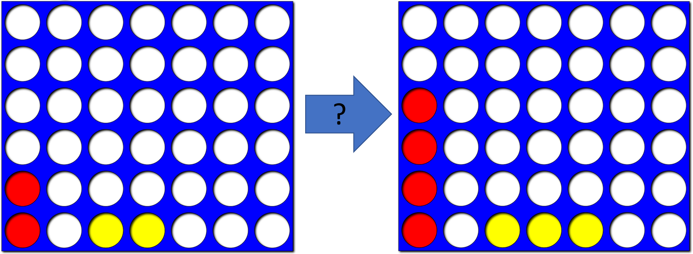
Should Red try to achieve the connect 4 shown on the right?
To evaluate Red’s next move, we look at the game tree:
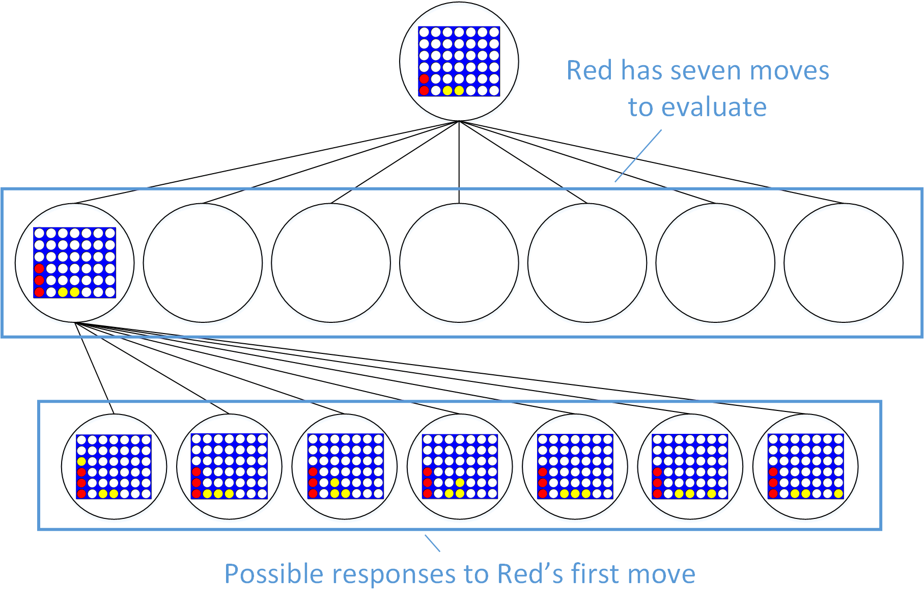
Partial game tree
Red has seven moves to choose from, only one of which may lead to the connect 4 that is on the right in Figure 3. To determine the strength of that move, we need to consider how Yellow can respond to it. Yellow’s first possible response blocks Red’s connect 4. The remaining six responses do not block Red’s connect 4, which would allow Red to win on the very next move. Only the first of these possible responses matters. If Yellow is playing well, he will block Red from winning by choosing the leftmost move.
For Red, this means the leftmost move should be evaluated as one that leads to Yellow blocking his connect 4, not as a move that will lead to an immediate victory. In other words, Red should evaluate each possible move by assuming that Yellow will respond with the move that is best for Yellow. This assumption that the opposing player will act in his own best interest is the heart of the minimax algorithm.
To turn this assumption into something a computer can implement, a score indicating the strength of each move needs to be calculated for each node of the game tree. Higher scores are better for Red, so Red tries to maximize the score. Lower scores are better for Yellow, so Yellow tries to minimize the score. One possible scoring system would be a scale from -21 to +21:
| Score | Meaning |
|---|---|
| 21 | Win for Red. |
| 20 | Very, very good situation for Red |
| … | |
| -20 | Very, very good situation for Yellow |
| -21 | Win for Yellow |
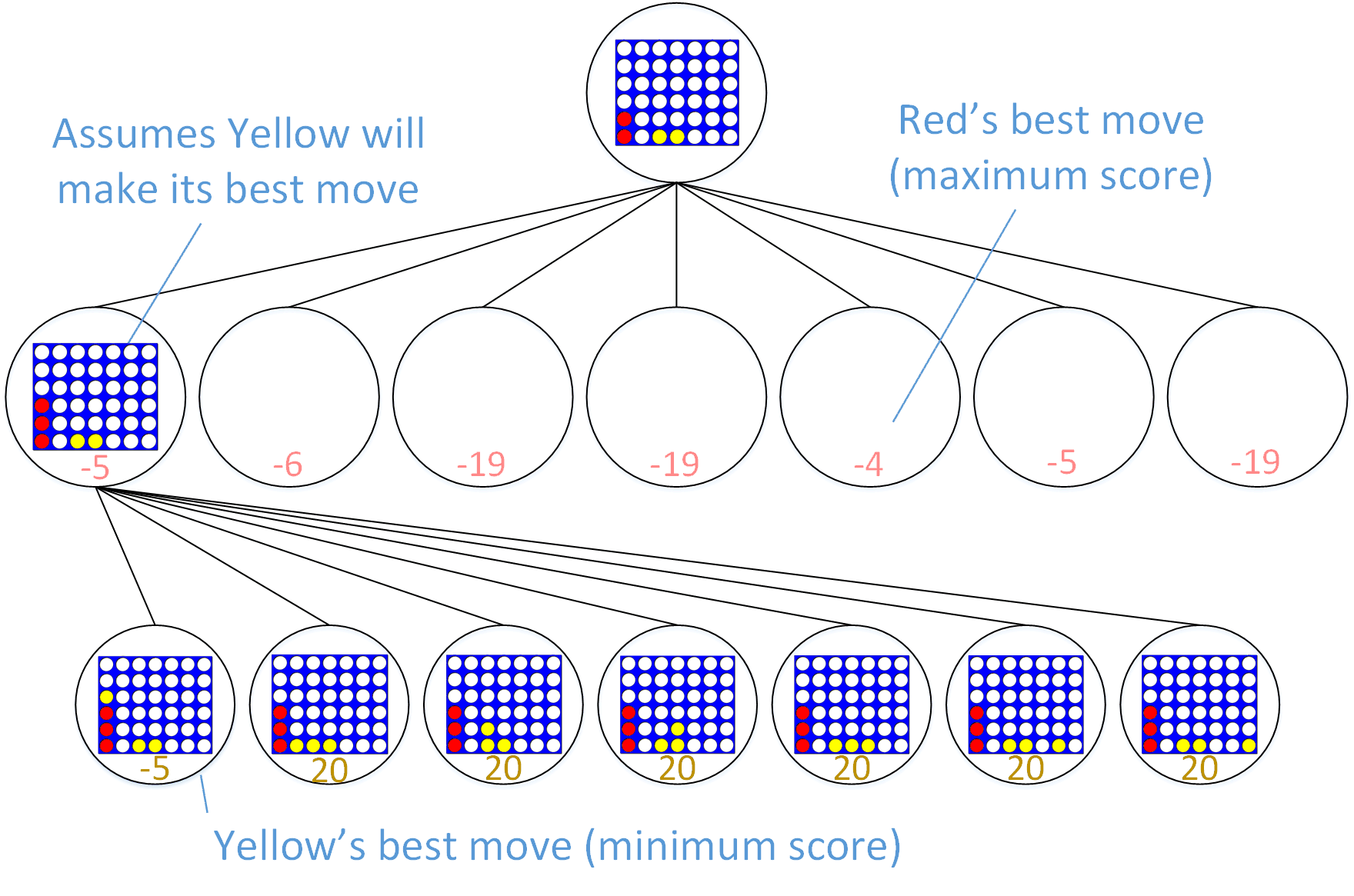
Let’s look at how we can use these scores to pick where Red should place his third game piece. Recall that Red is considering playing this piece in the leftmost column, as seen in the middle row of Figure 5. For Red to determine what score to give to this move, he looks at every move Yellow could make in response.
Yellow’s options for responding are shown in the bottom row of Figure 5. Yellow’s first option (column 1) results in a good situation for Yellow (score: -5). Yellow’s remaining options are very, very bad for Yellow (score: +20, because Red can win on the next move). Red assumes Yellow would choose his best response (score: -5), so Red’s first option (i.e. placing his piece in column 1) receives the same score (-5).
This score-calculation process repeats for each one of Red’s possible moves (i.e. columns 2-7, which are represented by the middle row in Figure 5). The result is a score for each one of Red’s options. Just as Yellow chooses the best score for Yellow, Red chooses the best score for Red. In this example, playing his piece in the fifth column has a better score for Red than the first column, so that is the move Red will choose.
Partial game tree
This process of evaluating and selecting moves by assuming that one player always minimizes the score and the other always maximizes the score is called minimax.
Calculating Scores Without Running Out of Memory
The process of calculating a perfectly accurate score is recursive. For example, to obtain the score (-5) of the lower left node in Figure 5, we need to look at every move Red could make in response to this game state. But scoring Red’s possible responses requires scoring every possible move Yellow could make in response to each of Red’s responses, and so on. The process only ends when we reach a game state that unambiguously leads to a win, loss, or draw. In short, computing the scores needed to select the best move requires constructing the entire game tree.
For Connect 4, the complete game tree contains more than four trillion nodes! The game tree is even larger in games such as Go. It is not feasible to construct the complete game tree for most games. Instead, the size of the game tree is limited, and scores are estimated rather than calculated.
The technique used by IBM’s Deep Blue was to explore the game tree up to a set depth (e.g. 6 moves by each player). When that depth was reached, a heuristic was used to assign an estimated score to each of the nodes at the bottom of the tree. Those estimated scores were used by the minimax move selection algorithm to assign scores to each of the higher-level nodes in the game tree and select a move. The process of generating game-specific heuristics is beyond the scope of this post.
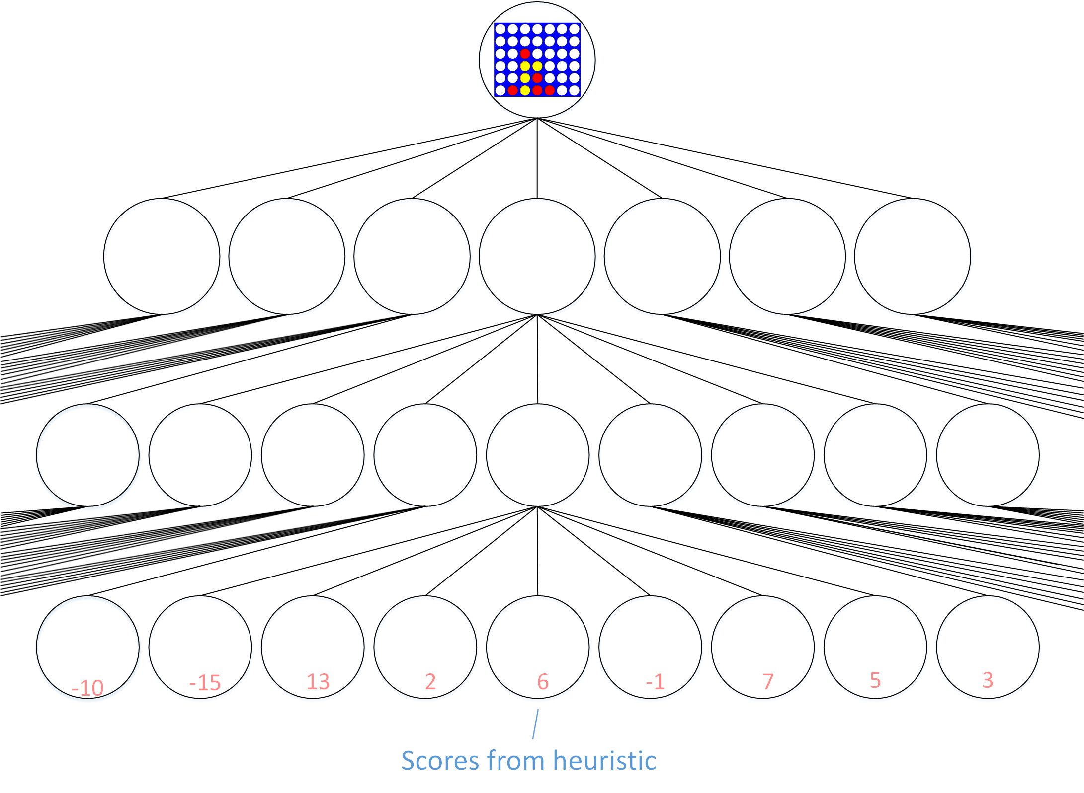
Game engines expand the game tree to a preset depth and then use a heuristic to assign scores
If it were feasible to obtain perfectly accurate scores, the minimax move selection algorithm would result in perfect play. Deep Blue explored the game tree as much as possible before resorting to its score-estimating heuristic. This was vastly better than relying on the heuristic alone. But the inaccuracies in the score-estimating heuristic nonetheless resulted in very close matches against Garry Kasparov. In 1996 there were two draws, and Deep Blue lost three of the remaining four games to Kasparov. In 1997 there were three draws, and Deep Blue lost one of the remaining three games.1
As explained in the next post, Monte Carlo techniques may be used if the programmer cannot provide a reasonable score-estimating heuristic.
Alpha-Beta Pruning – A Minimax Optimization
Deep Blue also used an optimization called alpha-beta pruning. This technique “prunes” unpromising branches from the game tree. This frees up memory and processing time for additional exploration of the more promising branches of the game tree. For example, if the player seeking to maximize the score has to pick between a node whose estimated score is 15 and a node whose estimated score is only 1, the player would never choose the unpromising node whose estimated score is only 1. Consequently, the branch of the game tree that lies below the unpromising node is “pruned”—it is not explored any further.
Monte Carlo Tree Search techniques inherently achieve a similar optimization. Although Monte Carlo techniques do not completely ignore any branch, unpromising branches are explored less and promising branches are explored more.
Conclusion
Thanks for reading! Don’t forget to continue to the discussion of Monte Carlo Tree Search!